|
The Art of Demomaking - Issue 11 - Particle Systems by (01 November 1999) |
Return to The Archives |
Introduction
 |
|
This week we make the big jump into the world of 3D... so you'd better hold on to your mouse and keyboard because this is the part that gets really interesting. First of all I will give you the basic knowledge you need to understand 3D programming, and I will show you how useful matrices are. Then we will apply all that to create a particle system. And to polish off our effect, you will see how to anti-alias pixels and how to use feedback with image rescaling. |
|
The World In Three Dimensions
|
|
The world we evolve in is based on 3 dimensions. You can picture that as a 2D graph with an extra Z axis. There are different conventions to orientate the axes, but only one makes sense. Hold out your left hand in front of you, pointing forwards. Your thumb points upwards, and your middle finger points to the right. By convention, your middle finger points towards positive X, the index finger points towards positive Z, and the thumb points towards positive Y. In this world we can define vertices. These are just points that have 3 components that can each be projected onto these 3 axes. Vertices have no direction. Vectors on the other hand are by definition a direction. Vectors are the difference of two vertices, hence they point from one to the other. Vectors don't have a fixed origin, so they apply to any point in 3D space. You can of course represent a vector with a vertex, by assuming the second point in question is at the origin. So in essence, we only need one data structure to store both these types. Vertices are usually defined in world space. Which means they are in a predefined coordinate system, which you chose when you create your world. The aim of the 3D application is to find the coordinates of these vertices in camera space, by rotating and translating them as necessary. Then from camera space we must convert to screen space by projecting them. |
|
The Matrix
|
|
The Matrix is all around you. It is in the air you breathe, erm... no! Wrong matrix. The matrix we're interested in is just a two dimensionnal array, usually 3x3 or 4x4. 4x4 matrices can represent any transformation from 3D to 3D. They are also a superset of 3x3 matrices, so you can perform any 3x3 matrix operation with a 4x4 matrix. A 3x3 matrix is sufficient to represent the coordinate system we talked about in the previous section. The first column in the matrix represents the x axis of the local coordinate system, the second column represents the y axis, and the third column the z axis. 4x4 matrices can also store the origin of the coordinate system, which explains why 4x4 matrices can also handle translations, where as 3x3 matrices are pretty much limited to rotations. 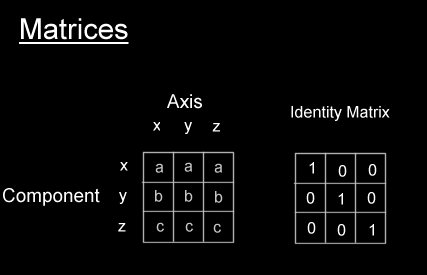 Notice the very special identity matrix. This matrix aligns perfectly with the world coordinates that we defined above, so no operations need to be performed to transform the vertices in the world to camera space. Now the only thing we need to know is how to use these matrices to perform our 3D operations for us. The trick is simple, we compose our camera matrix by multiplying several sub-matrices containing the separate transformations, like so:
We could also add translation, scaling, and projection if we wanted. Note that matrix multiplication is not commutative, so the order in which you multiply them is very important. Matrix multiplication is done like this:
Once we have our transformation matrix, we must transform our vertices by applying them to the following procedure:
And that's all you need to convert your vertices in object space to camera space. But there's still one more stage to go. |
|
Converting 3D to 2D
|
Now we need to display this 3D data on our 2D screens. To do this we model the screen as a plane in the 3D world, that's the projection plane. So to convert a 3D coordinate to 2D we just project the vertex onto this plane. This is just like following an imaginary ray towards the camera, until we hit this plane. 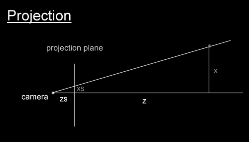 zs is the distance from the camera to the projection plane. z is the distance from the camera to the orthogonal projection of the point on the z axis. So given this figure, we know thanks to Thales that
We also have to add two constants to centre the coordinate system in the middle of our screen. So the equation ends up more like:
Now all we need to do is draw something on the screen at that location. |
|
Antialiasing Pixels
|
Now we have the screen coordinates of our particles, we can draw them. We want to avoid simply drawing to the closest pixel, since this doesn't look too good, and the movement seems jagged. So we use simple antialiasing to draw the pixels. Some of you may know this technique as Wu pixels.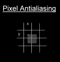 The theory is we set the colour of the real pixels proportionally to the area of the theoretical pixels that's inside. It involves a few more multiplications, and 4 memory writes, but it's well worth the output quality boost. The following code will draw the antialiased pixels:
You could also draw the particles as flares, or any kind of sprites. But the nicest results are produced when you add the intensity of each particle to the screen. Don't forget to check for overflow if you do that. |
|
Image Rescaling
|
|
This is a simple technique that looks extremely good. The idea is that we use the previous frame and copy a small portion of it which we scale to size and blur. We then draw the current frame over the top. This can produce some cool light effects, like when a flash-light shines through the fog. The following code finds the distance of each pixel to a certain point, and scales that distance to find which pixel to copy from.
This code can be quite significantly optimised. You could also add some simple sine modulation to that, which can produce some unexpected results ;) |
|
Final words
|
|
Once you get addicted to 3D coding, you'll find it quite difficult to go back to 2D effects. Just keep in mind that most great effects combine both 2D and 3D, all in one. Next week I will take you further on this fascinating expedition into the world of 3D. Again I can't give you a detailed map of where we are going, since I don't know myself. Rest assured that I will make sure it's safe before I take you there though ;) Feel free to download this week's example and source code package right here (68k) Have fun, Alex |